Overview
FreightWaves Benchmark Spot Rates provide a cost-based model for setting spot rates for more than 735,000 zip3 origin-destination pairs greater than 250 miles in the contiguous United States. They are based on an empirically derived conceptual model that accounts for market conditions, including tender data, toll data, several other miscellaneous variables, and aggregated carrier expense data. This model provides a rational starting place to discover the historic trend in spot rates, a cost-based anchor for today’s rate, and an artificial intelligence-driven forecast of where rates are headed in the future.
The FreightWaves data science team uses historical market and anonymized expense data to forecast future market conditions, so that FreightWaves Benchmark Spot Rates can be calculated for future dates. This assists customers in understanding the effects that coming changes in markets might have on spot rates, and aids in both short- and long-term decision-making. The model is shown below, with the major input variables to the model shown above the FreightWaves Benchmark Spot Rates for those market conditions.
Because FreightWaves Benchmark Spot Rate Forecasts are based on the forecasts of underlying market conditions, the accuracy of the forecasts is determined by comparing the forecasts with the FreightWaves Benchmark Spot Rates generated using real-time market conditions. The accuracy for a six-month forecast for Thanksgiving and Christmas 2019 is analyzed below, as well as a set of forecasts for national and regional rates made at one-week, one-month and three-month horizons during the period between May 1 and June 15, 2020.
The FreightWaves data science team is analyzing how accurate the forecasting tool is at forecasting itself. It is not being compared to anything else. The rates are largely dependent on truckload supply and demand metrics. The forecasted supply and demand metrics are used to calculate the forecasted rates. For example, FreightWaves compares the forecasted rate from one month ago, which is based on forecasted supply and demand metrics, to today’s rate, which is based on actual supply and demand metrics.
The forecasted rates are benchmark rates that provide a representation of market conditions. This shows how accurate the FreightWaves data science team is at predicting future market conditions, displayed as benchmark rates.
The accuracy of the FreightWave’s benchmark spot rate forecasts are described below. They include the accuracy of a six-month forecast for Thanksgiving and Christmas 2019, and an analysis that displays the results from 135 models for a complete 1.5-month period between May 1 and June 15, 2020 at one-week (7 days), one-month (28 days) and three-month (84 days) forecast horizons.
Summary of findings
Among the observations to-date are:
- The forecast models continually learn and improve over time (Figures 1 and 2).
- For the 2019 holiday season and for models built using one holiday season for training, the national-level percentage of error at a six-month horizon is 8.64% for Thanksgiving and 11.81% for Christmas (Figure 1).
- For the 2019 holiday season and for models built using two holiday seasons for training, the national-level hypothetical percentage error (using the 2019 holiday season as the “actuals”) at a six-month horizon is 5.11% for Thanksgiving and 10.64% for Christmas (Figure 2).
- For the 2019 holiday season at a region-to-region level, the models captured the level, trend and seasonality well (Figures 3 and 4).
- For the time period May 1, 2020 to June 15, 2020 at a national level, the average percentage error for a 7-day horizon, 28-day horizon and 84-day horizon are 5.56%, 5.63% and 5.39% respectively (Figure 5).
- The errors are similar between regions for the time period May 1, 2020 to June 15, 2020 (Figure 6).
Six month outlook: 2 models built in 2019 and 2 models built in 2020
Figure 1
Six-month national outlook for Thanksgiving (brown dashed line) and Christmas 2019 (red and green dashed line) using two forecasting models with only one holiday season (2018) in the training data. The black line is the actual Benchmark rate. Arrows indicate six months from when the model was trained. The model build-dates are indicated by the back dashed lines: one built on June 1, 2019 (180 days prior to Thanksgiving) and one built on June 28, 2019 (180 days prior to Christmas). The models capture the seasonality but do a poor job of capturing the absolute rate levels.
Figure 2
Six-month national outlook for Thanksgiving (brown dashed line) and Christmas 2019 (red and green dashed line) and using two forecasting models with two holiday seasons (2018 and 2019) in the training data. The black line is the actual Benchmark rate. The models were built for June 1, 2020 and June 28, 2020, and the forecast for the 2020 holiday season is superimposed on the 2019 holiday season. The models capture both the seasonality and result in improved estimates of the absolute rate values.
Figure 3
Six-month regional outlook for Thanksgiving (brown dashed line) and Christmas 2019 (red and green dashed line). The black line is the actual Benchmark rate. Two model forecasts are shown: one built on June 1, 2019 (180 days prior to Thanksgiving) and one built on June 28, 2019 (180 days prior to Christmas).
Figure 4
Six-month regional outlook for Thanksgiving (brown dashed line) and Christmas 2019 (red and green dashed line) using two forecasting models with two holiday seasons (2018 and 2019) in the training data. The black line is the actual Benchmark rate. The models were built for June 1, 2020 and June 28, 2020 and the forecast for the 2020 holiday season is superimposed on the 2019 holiday season. The models capture the seasonality and result in improved estimates of the absolute rate values.
Three-month, one-month and one-week outlook: 135 models built in 2020
Figure 5
Forecasted vs. observed for nationally aggregated rates. 135 model forecasts were used to generate this plot (3 models per day for 45 days). The black line is the average of rates weighted by the outbound tender volume for the origin and the inbound tender volume for the destination.
Figure 6
Forecasted vs. observed for regionally aggregated rates. 135 model forecasts were used to generate this plot (3 models per day for 45 days). The black line is the average of rates weighted by the outbound tender volume for the origin and the inbound tender volume for the destination.
Legal disclaimer
The benchmark spot rates are the result of an exploratory analysis and FreightWaves does not guarantee the accuracy, availability, completeness or usefulness of the information at this time. However, due to the promising data generated to date, FreightWaves will continue to refine this material for broader use going forward.


